Use
Processing a video
A description of the GUI components referred to here is given in the ''GUI description'' section.
Steps:
- Load the GUI from the command line or by double-clicking on the Safas shortcut, as described in the Installation section. The initial GUI window will be loaded, refer to Fig. 1. To load Safas from the command line:
$ conda activate safas_env
(safas_env) $ safas
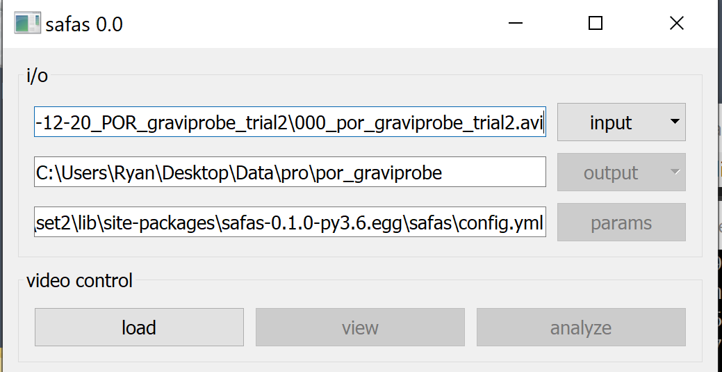
Fig. 1: Main panel
- There are three ways to select a parameters file: (1) pass the file name to Safas on the command line; (2) let the software load a default file from the module; or (3) set the config file interactively in the Main panel by clicking the
paramsbutton. - Note: after you have completed one analysis, an updated config file will be saved to the output directory and you can use that file as a starting point for your next analysis.
- Click
input > file, then select your video file. - Click
output, to select location of the output directory. If 'baseout' has been set in the 'config.yml', the data will be saved relative to that path. - Click
load-- to set the parameters and check inputs -- thenviewto load the video viewer. - The
loadbutton will change toreleaseand can be pushed to close the viewer or load a new video. - The slider at the bottom of the video viewer, refer to the right hand window of Fig. 2, may be used to scroll or ''scrub'' through the video.
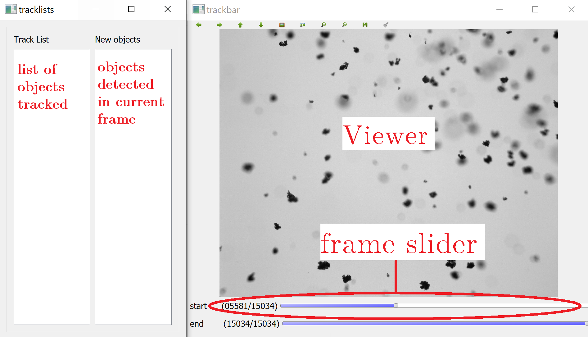
Fig. 2: Video viewer
- Click
Analyzeto load thetracking panelGUI for access to image processing and object tracking tools. - On the
tracking panelthere are several tools including: setting image filter parameters, tracking objects, saving plotting, merging data sets, refer to Fig. 4.

Fig. 3: Tracking panel
-
To change the filter parameters, click
filter paramsin the image filter box. A panel to interactively set the image filter parameters will appear. Adjust the sliders and radio buttons, then pressTestto check the result. -
Carefully inspect the processed image. Are the flocs segmented properly? Zoom in and out with the magnifying glass or ctrl + mouse wheel. To improve the segmentation results, test different combinations of filters and parameters by loading the image filter parameters dialog.
-
When satisfied, press
Saveto save the parameters, then pressExit.

Fig. 4: Filter panel
- On the
tracking panel, click theprocess img.radio button toon, then press theNext frame >. The processed image will be displayed and if there are any in focus objects, they will be outlined in green and listed in theNew objectslist, refer to Figure 5.
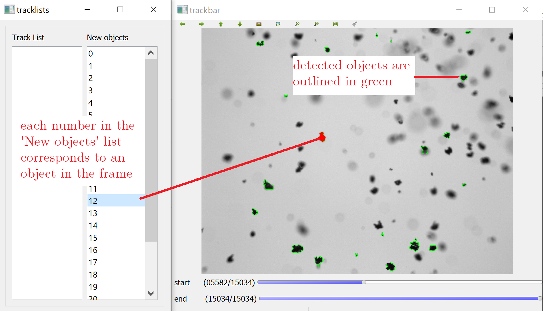
Fig. 5: Processed image
-
If you decide to select a new region to analyze, click the
process img.radio button tooff, then scrub to a new location in the video. Pressonagain, to re-start processing the images. -
Click on the
New objectslist panel. Press the up and down keys on the keyboard to highlight different objects. The current object will also be highlighted in the viewer. Note that smaller objects may be harder to see. To improve the visualization of small objects, you may open the image filter parameters dialog and increase the contour width. - With the
New objectspanel active, press theakey on the keyboard to add the current object to the analysis. You will see a new number added to theTrack List.Add as many objects as you would like, avoid poorly segmented objects but ensure to sample a wide variety of sizes. - To track the selected objects, press the
nkey on the keyboard or press thenext frame >button. The integer value in thestep int.text box is the number of frames the objects will be tracked through. - The object tracks will be displayed in the viewer, refer to an example in Fig. 6. Note that some objects may not be correlated in one of the frames and will be ''lost.'' If this happens, the software will ''terminate'' the track of that object.
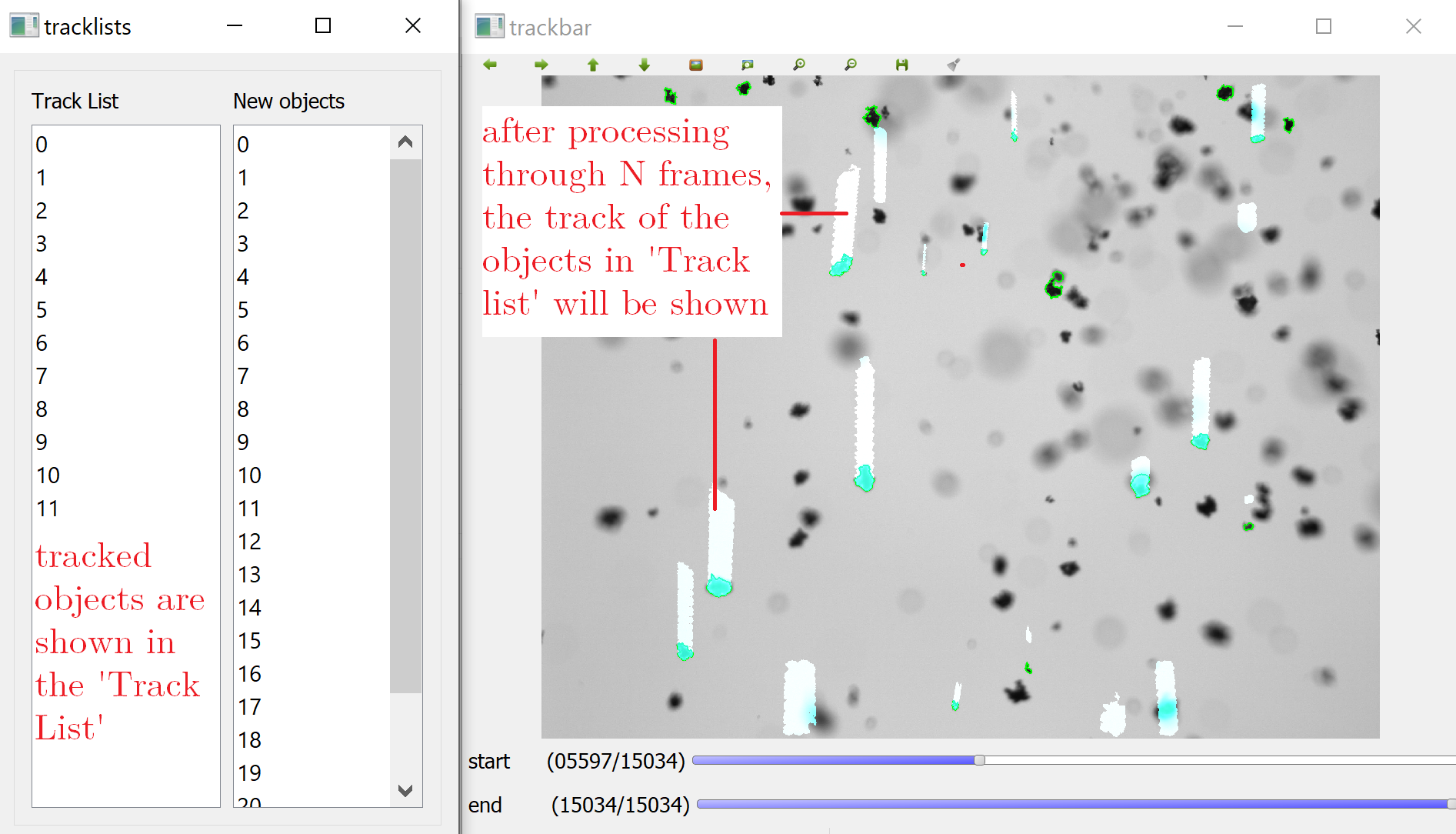
Fig. 6: Tracked objects
- Click
saveto export the results as an .xlsx file. The morphological properties and velocity data of the objects will be saved. - In most cases, the user will want to analyze several sections of the video. Here are several suggestions to improve the workflow in this case:
- Let the software automatically name the output as ''floc_props_frame_NNNNN.xlsx'' where NNNNN is the number of the last frame analyzed.
- Turn
Confirm properties after each save?toOff. - Turn
Clear data after savetoOn. Otherwise, you will need to clear the tracks manually.

Fig. 7: Save panel
- Move the trackbar to a new position in the video and continue the analysis.
- After analyzing several sections of video, press the
mergebutton to select the files that will be compiled into a single .xlsx file. - Consider plotting the results immediately to ensure an adequate sampling of objects has been achieved.
- Click
plotand select variables to plot on the x- and y-axes, refer to Fig. 8. The plot window has several built in features for changing the axis appearance and scaling. - Press the
savebutton to save the data to the output directory.

Fig. 8: Plot panel
- Press
releasein the main panel to load another video or exit the program with thexin the top right-hand corner.
Filters and Modules
Several components of Safas may be used directly in a Python script of Jupyter notebook. There are several examples in the Safas repo under ''notebooks.''
For example ''notebooks/sobel_focus_example.ipynb'' and ''notebooks/segmentation_with_noisy_background.ipynb'' demonstrate how to use the filters directly; while ''notebooks/tracking_criteria.ipynb'' demonstrates the use of the ''matcher'' module for object correlation.